Error-Correcting Codes

We will consider two situations in which we wish to convey information on an unreliable channel. The first is exemplified by the internet, where the information (say a file) is broken up into packets, and the unreliability is manifest in the fact that some of the packets are lost (or erased) during transmission. Moreover the packets are labeled with headers so that the recipient knows exactly which packets were received and which were dropped. We will refer to such errors as erasure errors. See the figure below:

In the second situation, some of the packets are corrupted during transmission due to channel noise. Now the recipient has no idea which packets were corrupted and which were received unmodified:

In the above example, packets \(1\) and \(4\) are corrupted. These types of errors are called general errors. We will discuss methods of encoding messages, called error-correcting codes, which are capable of correcting both erasure and general errors. The principle is to embed a message into a codeword (a process called encoding), transmit the codeword, and then recover the message from the damaged/corrupted symbols that are received (a process called decoding).

This area of study is a part of “Information Theory,” one of the core computer sciences¹ along with the theory of computation, control theory, communication theory, and estimation/learning theory. At the National Science Foundation, these are (largely) currently in the Computer and Information Science and Engineering (CISE) directorate in the Division of Computing and Communication Foundations (CCF). In particular, there is a rich area of coding theory and here in this note, we will simply touch a little part of it. If you want to learn more, this material is built upon in 121, 229A, 229B, and other courses.

On the practical side, this material is intensely useful. Every time you use your cellphone, satellite TV, DSL, cable-modem, hard-disk drive, solid-state drive, CD-ROM, DVD, Blu-ray, etc., error-correcting codes are crucial. Related ideas are being deployed in the Internet for streaming and in modern data-centers to make cloud computing and distributed storage possible. Perhaps most surprisingly, the actual (polynomial-based) codes that you are studying in this lecture notes are called Reed-Solomon² codes and are essentially what are used in many applications. These are representative of what are called algebraic-geometry codes, because of their connections to algebraic geometry — the branch of mathematics that studies the roots of polynomial equations.

Returning to the problem at hand. Assume that the information consists of \(n\) packets³ . We can assume without loss of generality that the contents of each packet is a number modulo \(q\) (denoted by \(\operatorname{GF}(q)\)), where \(q\) is a prime. For example, the contents of the packet might be a \(32\)-bit string and can therefore be regarded as a number between \(0\) and \(2^{32} -1\); then we could choose \(q\) to be any prime⁴ larger than \(2^{32}\). The properties of polynomials over \(\operatorname{GF}(q)\) (i.e., with coefficients and values reduced modulo \(q\)) are the backbone of both error-correcting schemes. To see this, let us denote the message to be sent by \(m_1 , \ldots, m_n\) and make the following crucial observations:

1) There is a unique polynomial \(P(x)\) of degree \(n - 1\) such that \(P(i) = m_i\) for \(1 \leq i \leq n\) (i.e., \(P(x)\) contains all of the information about the message, and evaluating \(P(i)\) gives the intended contents of the \(i\)-th packet).

2) The message to be sent is now \(m_1 = P(1), \ldots, m_n = P(n)\). We can generate additional packets by evaluating \(P(x)\) at additional points \(n+1, n+2, \ldots, n+j\) (remember, our transmitted codeword must be redundant, i.e., it must contain more packets than the original message to account for the lost or corrupted packets). Thus the transmitted codeword is \(c_1 = P(1) , c_2 = P(2) , \ldots , c_{n+j} = P(n+j)\). (Alternatively, we can use the \(n\) numbers defining the message as the coefficients of a degree \(n-1\) polynomial directly. Either way, the transmitted codeword will be evaluations of this polynomial.) Since we are working modulo \(q\), we must make sure that \(n + j \leq q\), but this condition does not impose a serious constraint since \(q\) is presumed to be very large.

Erasure Errors

Here we consider the setting of packets being sent over the internet. In this setting, the packets are labeled and so the recipient knows exactly which packets were dropped during transmission. One additional observation will be useful:

3) By Property 2, we can uniquely reconstruct \(P(x)\) from its values at any \(n\) distinct points, since it has degree \(n-1\). This means that \(P(x)\) can be reconstructed from any \(n\) of the transmitted packets. Evaluating this reconstructed polynomial \(P(x)\) at \(x = 1, \ldots , n\) yields the original message \(m_1 , \ldots , m_n\). (Or alternatively, if the message was encoded into the polynomial’s coefficients, we could just read the message out by simplifying the polynomial.)

Recall that in our scheme, the transmitted codeword is \(c_1 = P(1) , c_2 = P(2) , \ldots , c_{n+j} = P(n+j)\). Thus, if we hope to be able to correct \(k\) errors, we simply need to set \(j= k\). The encoded codeword will then consist of \(n + k\) packets.

Example

Suppose Alice wants to send Bob a message of \(n=4\) packets and she wants to guard against \(k=2\) lost packets. Then, assuming the packets can be coded up as integers between \(0\) and \(6\), Alice can work over \(\operatorname{GF}(7)\) (since \(7\ge n+k = 6\)). Suppose the message that Alice wants to send to Bob is \(m_1 = 3\), \(m_2 = 1\), \(m_3 = 5\), and \(m_4 = 0\). She interpolates to find the unique polynomial of degree \(n - 1 = 3\) described by these 4 points: \(P(x) = x^3 + 4x^2 + 5\) (verify that \(P(i) = m_i\) for \(1 \leq i \leq 4\)).

Since \(k=2\), Alice must evaluate \(P(x)\) at \(2\) extra points: \(P(5) = 6\) and \(P(6) = 1\). Now, Alice can transmit the encoded codeword which consists of \(n + k = 6\) packets, where \(c_j = P(j)\) for \(1\leq j \leq 6\). So \(c_1 = P(1) = 3\), \(c_2 = P(2) = 1\), \(c_3 = P(3) = 5\), \(c_4 = P(4) = 0\), \(c_5 = P(5) = 6\), and \(c_6 = P(6) = 1\). Suppose packets \(2\) and \(6\) are dropped, in which case we have the following situation:

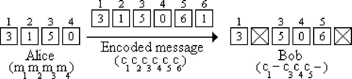
From the values that Bob received (\(3\), \(5\), \(0\), and \(6\)), he uses Lagrange interpolation and computes the following delta functions: \[\begin{aligned} \Delta_1(x) &= \frac{(x - 3)(x - 4)(x - 5)}{-24}\\ \Delta_3(x) &= \frac{(x - 1)(x - 4)(x - 5)}{4}\\ \Delta_4(x) &= \frac{(x - 1)(x - 3)(x - 5)}{-3}\\ \Delta_5(x) &= \frac{(x - 1)(x - 3)(x - 4)}{8}.\end{aligned}\] He then reconstructs the polynomial \(P(x) = (3)\Delta_1(x)+(5)\Delta_3(x)+(0)\Delta_4(x) + (6)\Delta_5(x) = x^3 + 4x^2 + 5\). Bob then evaluates \(m_2 = P(2) = 1\), which is the packet that was lost from the original codeword. More generally, no matter which two packets were dropped, following the same method Bob could still have reconstructed \(P(x)\) and thus the original message.

Let us consider what would happen if Alice sent one fewer packet. If Alice only sent \(c_j\) for \(1 \leq j \leq n + k - 1\), then with \(k\) erasures, Bob would only receive \(c_j\) for \(n - 1\) distinct values \(j\). Thus, Bob would not be able to reconstruct \(P(x)\) (since there are exactly \(q\) polynomials of degree at most \(n - 1\) that agree with the \(n - 1\) packets which Bob received). This error-correcting scheme is therefore optimal: it can recover the \(n\) characters of the message from any \(n\) received characters, but recovery from any fewer characters is impossible.

Polynomial Interpolation

Let us take a brief digression to discuss another method of polynomial interpolation which will be useful in handling general errors. The goal of the algorithm will be to take as input \(d+1\) pairs \((x_1,y_1),\ldots,(x_{d+1},y_{d+1})\), and output the polynomial \(p(x) = a_dx^d + \cdots + a_1x + a_0\) such that \(p(x_i) = y_i\) for \(i = 1\) to \(d+1\).

The first step of the algorithm is to write a system of \(d+1\) linear equations in \(d+1\) variables: the coefficients of the polynomial \(a_0, \ldots, a_d\). Each equation is obtained by fixing \(x\) to be one of \(d+1\) values: \(x_1,\ldots,x_{d+1}\). Note that in \(p(x)\), \(x\) is a variable and \(a_0,\dots,a_d\) are fixed constants. In the equations below, these roles are swapped: \(x_i\) is a fixed constant and \(a_0,\dots,a_d\) are variables. For example, the \(i\)-th equation is the result of fixing \(x\) to be \(x_i\): \(a_d x_i^d + a_{d-1} x_i^{d-1} + \cdots + a_0 = y_i\).

Now solving these equations gives the coefficients of the polynomial \(p(x)\). For example, given the \(3\) pairs \((-1,2)\), \((0,1)\), and \((2,5)\), we will construct the degree \(2\) polynomial \(p(x)\) which goes through these points. The first equation says \(a_2(-1)^2 + a_1(-1) + a_0 = 2\). Simplifying, we get \(a_2 - a_1 + a_0 = 2\). Similarly, the second equation says \(a_2(0)^2 + a_1(0) + a_0 = 1\), or \(a_0 = 1\). And the third equation says \(a_2(2)^2 + a_1(2) + a_0 = 5\). So we get the following system of equations: \[\begin{aligned} a_2 - a_1 + a_0 &= 2\\ a_0 &= 1\\ 4a_2 + 2a_1 + a_0 &= 5\end{aligned}\] Substituting for \(a_0\) and multiplying the first equation by \(2\) we get: \[\begin{aligned} 2a_2 - 2a_1 &= 2\\ 4a_2 + 2a_1 &= 4\end{aligned}\] Then, adding the two equations we find that \(6a_2 = 6\), so \(a_2 = 1\), and plugging back in we find that \(a_1 = 0\). Thus, we have determined the polynomial \(p(x) = x^2 + 1\). To justify this method more carefully, we must show that the equations always have a solution and that it is unique. This involves showing that a certain determinant is non-zero, which we will leave as an exercise⁵.

General Errors

Now let us return to general errors. General errors are much more challenging to correct than erasure errors. This is because packets are corrupted, not erased and Bob no longer knows which packets are correct. As we shall see shortly, Alice can still guard against \(k\) general errors, at the expense of transmitting only \(2k\) additional packets or characters (only twice as many as in the erasure case). Thus the encoded codeword is \(c_1, \ldots, c_{n+2k}\) where \(c_j = P(j)\) for \(1 \leq j \leq n + 2k\). This means that at least \(n+k\) of these characters are received uncorrupted by Bob.

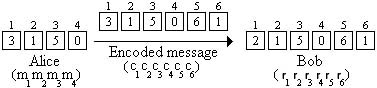
For example, if Alice wishes to send \(n = 4\) characters to Bob via a modem in which \(k = 1\) of the characters is corrupted, she must redundantly send a codeword consisting of 6 characters. Suppose she wants to convey the same message as above, and that \(c_1\) is corrupted and changed to \(r_1 = 2\). This scenario can be visualized in the following figure:

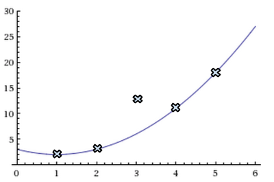
Bob’s goal is to reconstruct \(P(x)\) from the \(n+2k\) received symbols \(r_1,\ldots,r_{n+2k}\). He knows that \(P(i)\) must equal \(r_i\) on at least \(n+k\) points (since only \(k\) points are corrupted), but he does not know which of the \(n+k\) values are correct. As an example, consider a possible scenario depicted in the picture below. The points represent the symbols received from Alice, and the line represents \(P(x)\). In this example, \(n = 3\), \(k = 1\), and the third packet is corrupted. Bob does not know the index at which the received symbols and the polynomial deviate:

Bob attempts to construct \(P(x)\) by searching for a polynomial \(P'(x)\) with the following property: \(P'(i) = r_i\) for at least \(n+k\) distinct values of \(i\) between \(1\) and \(n+2k\). Of course, \(P(x)\) is one such polynomial. It turns out⁶ that \(P(x)\) is actually the only polynomial with the desired property. Therefore, \(P'(x)\) must equal \(P(x)\).

Finding \(P(x)\) efficiently requires a remarkable idea, which is just about simple enough to be described here. Suppose packets \(e_1,\dots,e_k\) are corrupted. Define the degree \(k\) polynomial \(E(x)\) to be \((x-e_1)\cdots(x-e_k)\). Let us make a simple but crucial observation: \[P(i)E(i) = r_iE(i) \mbox{ for }1 \leq i \leq n+2k\] (this is true at points \(i\) at which no error occurred since \(P(i) = r_i\), and trivially true at points \(i\) at which an error occurred since \(E(i) = 0\)).

This observation forms the basis of a very clever algorithm invented by Berlekamp and Welch. Looking more closely at these equalities, we will show that they can be cast as \(n+2k\) linear equations in \(n+2k\) unknowns. The unknowns correspond to the coefficients of \(E(x)\) and \(Q(x)\) (where we define \(Q(x) = P(x)E(x)\)). Once \(Q(x)\) and \(E(x)\) are known, we can divide \(Q(x)\) by \(E(x)\) to obtain \(P(x)\).

Since \(Q(x)\) is a polynomial of degree \(n+k-1\), it can be described by \(n+k\) coefficients. \(E(x)\) is a degree \(k\) polynomial, but its definition implies that its first coefficient must be \(1\). It can therefore be described by \(k\) coefficients: \[\begin{aligned} Q(x) = a_{n+k-1}x^{n+k-1} + \cdots + a_1x + a_0 \\ E(x) = x^k + b_{k-1}x^{k-1} + \cdots + b_1x + b_0\end{aligned}\] As seen in the interpolation method above, once we fix a value \(i\) for \(x\), \(Q(i)\) and \(E(i)\) are linear functions of the unknown coefficients \(a_{n+k-1},\cdots,a_0\) and \(b_{k-1},\cdots,b_0\) respectively. The received value \(r_i\) is also fixed. Therefore the equation \(Q(i) = r_iE(i)\) is a linear equation in the \(n+2k\) unknowns \(a_{n+k-1}, \ldots, a_0\) and \(b_{k-1}, \ldots, b_0\). We thus have at least \(n+2k\) linear equations, one for each value of \(i\), and \(n+2k\) unknowns. We can solve these equations and get \(E(x)\) and \(Q(x)\). We can then compute the ratio \(Q(x)/E(x)\) to obtain \(P(x)\).

Example

Suppose we are working over \(\operatorname{GF}(7)\) and Alice wants to send Bob the \(n = 3\) characters “\(3\)”, “\(0\)”, and “\(6\)” over a modem. Turning to the analogy of the English alphabet, this is equivalent to using only the first \(7\) letters of the alphabet, where \(a = 0, \ldots, g = 6\). So the message which Alice wishes for Bob to receive is “dag”. Then Alice interpolates to find the polynomial \[P(x) = x^2 + x + 1,\] which is the unique polynomial of degree \(2\) such that \(P(1) = 3\), \(P(2) = 0\), and \(P(3) = 6\).

She needs to transmit the codeword consisting of \(n + 2k = 5\) characters \(P(1) = 3\), \(P(2) = 0\), \(P(3) = 6\), \(P(4) = 0\), and \(P(5) = 3\) to Bob. Suppose \(P(1)\) is corrupted, so he receives \(2\) instead of \(3\) (i.e., Alice sends the encoded codeword “dagad” but Bob instead receives “cagad”). Summarizing, we have the following situation:

Let \(E(x) = x + b_0\) be the error-locator polynomial—remember, Bob doesn’t know what \(b_0\) is yet since he doesn’t know where the (single) error occurred. Let \(Q(x) = a_3x^3 + a_2x^2 + a_1x + a_0\). Now Bob just substitutes \(x = 1, x = 2, \dotsc, x = 5\) into \(Q(x) = r_xE(x)\) and simplifies to get five linear equations in five unknowns. Recall that we are working modulo \(7\) and that \(r_i = c_i'\) is the value Bob received for the \(i\)th character.

The first equation will be \(a_3 + a_2 + a_1 + a_0 = 2(1 + b_0)\), which simplifies to \(a_3 + a_2 + a_1 + a_0 + 5b_0 = 2\). Bob can determine the remaining equations in the same manner, obtaining:

Then clearly \[P(x)E(x) = R(x)E(x)\] for \(x = 1, 2, \ldots, 5\) (if the corruption occurred at position \(i\), then \(E(i) = 0\), so equality trivially holds, and otherwise \(P(i) = R(i) = c'_i\)). Bob doesn’t know what \(P\) is (though he does know it is a degree \(2\) polynomial) and he doesn’t know what \(E\) is either, but using the relationship above he can obtain a linear system whose solutions will be the coefficients of \(P\) and \(E\), as seen below.

Let \[Q(x) = a_3x^3 + a_2x^2 + a_1x + a_0 = P(x)E(x),\] where \(a_3, a_2, a_1, a_0\) are unknown coefficients (which Bob will soon try to determine), so \[a_3x^3 + a_2x^2 + a_1x + a_0 = R(x)E(x) = R(x)(x - e_1),\] which he can rewrite as \[a_3x^3 + a_2x^2 + a_1x + a_0 + R(x)e_1 = R(x)x.\]

\[\begin{aligned} a_3 + a_2 + a_1 + a_0 + 5b_0 &= 2 \\ a_3 + 4a_2 + 2a_1 + a_0 &= 0 \\ 6a_3 + 2a_2 + 3a_1 + a_0 + b_0 &= 4 \\ a_3 + 2a_2 + 4a_1 + a_0 &= 0 \\ 6a_3 + 4a_2 + 5a_1 + a_0 + 4b_0 &= 1\end{aligned}\]

Bob then solves this linear system and finds that \(a_3 = 1,\) \(a_2 = 0,\) \(a_1 = 0,\) \(a_0 = 6,\) and \(b_0 = 6\) (all mod \(7\)). (As a check, this implies that \(E(x)=x+6=x-1\), so the location of the error is position \(e_1=1\), which is correct since the first character was corrupted from a “d” to a “c”.) This gives him the polynomials \(Q(x) = x^3 + 6\) and \(E(x) = x - 1\). He can then find \(P(x)\) by computing the quotient \[P(x) = \frac{Q(x)}{E(x)} = \frac{x^3 + 6}{x - 1} = x^2 + x + 1.\] Bob notices that the first character was corrupted (since \(e_1 = 1\)), so now that he has \(P(x)\), he just computes \(P(1) = 3 =\) “d” and obtains the original, uncorrupted message “dag”.

It is very informative to try doing this example yourself with some modifications. What happens if instead of changing the first character, we changed the second character? Do this and notice that everything still works.

What happens if we don’t change any character at all? In other words, we think that there might be a single error, but there isn’t any error. This is something worth doing on your own ahead of lecture, and then look at the footnote here⁷ for commentary. What happens if you change two characters instead of just one?

Finer Points Regarding Berlekamp-Welch

Two points need further discussion. How do we know that the \(n + 2k\) equations are consistent? What if they have no solution? This is simple. The equations must be consistent since \(Q(x) = P(x)E(x)\) together with the true error locator polynomial \(E(x)\) gives a solution, as long as there are exactly \(k\) errors.

Now, from the perspective of what we know about systems of linear equations, we have only ruled out the possibility of there being no solution. With \(n+2k\) equations and \(n+2k\) unknowns, the possibilities are that we have exactly \(1\) solution or many solutions.

So, the core interesting question is this: how do we know that the \(n + 2k\) equations are independent, i.e., how do we know that there aren’t many other spurious solutions in addition to the correct solution that we are looking for? Put more mathematically, how do we know that a solution \(Q'(x)\) and \(E'(x)\) that we reconstruct satisfies the property that \(E'(x)\) divides \(Q'(x)\) and that \[\frac{Q'(x)}{E'(x)} = \frac{Q(x)}{E(x)}= P(x)?\]

How to check that a ratio is the same? Use “cross products” from elementary school!

We claim that \(Q(x)E'(x) = Q'(x)E(x)\) for \(1\leq x\leq n + 2k\). This is a statement about evaluations of these polynomials. Since the degree of both \(Q(x)E'(x)\) and \(Q'(x)E(x)\) is \(n + 2k - 1\) and they are equal at \(n + 2k\) points, it follows from Property 2 that they are the same polynomial. Once we know that they are the same polynomial, we can divide both sides by the polynomial \(E(x)E'(x)\) since that polynomial is by construction not the zero polynomial. Rearranging, we get \[\frac{Q'(x)}{E'(x)} = \frac{Q(x)}{E(x)}= P(x).\]

So, it all hinges on the claim that \(Q(x)E'(x) = Q'(x)E(x)\) for all \(1\leq x\leq n + 2k\). Why is this claim true for these values? Based on our method of obtaining \(Q'(x)\) and \(E'(x)\), we know that \(Q'(i) = r_iE'(i)\) and \(Q(i) = r_iE(i)\). Now assume \(E(i)\) is \(0\). Then \(Q(i)\) is also \(0\), so both \(Q(i)E'(i)\) and \(Q'(i)E(i)\) are \(0\) and the claim holds. The same reasoning applies when \(E'(i)\) is \(0\).

That leaves the case when both \(E(i)\) and \(E'(i)\) are not \(0\). In this case, we are free to divide by it. So, we get \[\frac{Q'(i)}{E'(i)} = r_i\] and also \[\frac{Q(i)}{E(i)} = r_i.\] Since they are both equal to \(r_i\), they are equal to each other. So we get \[\frac{Q'(i)}{E'(i)} = \frac{Q(i)}{E(i)}.\] Doing cross-products (multiplying both sides of the equation by \(E(i)E'(i)\) and simplifying) now gives us the claim. Since the claim is now proven for all cases, it holds for all \(1 \leq x \leq n+2k\).

This means that when there are multiple solutions, they all point to the same polynomial, and hence to the same message. As you saw from playing around with the example, this actually happens when there are fewer errors than budgeted for.

Distance Properties

So far, we have talked about the Reed-Solomon codes in a way that constantly references their polynomial-evaluation based nature. However, it is useful to step back and ask ourselves what generic features of the codewords enabled us to recover from erasures and general errors.

It is useful here to treat a codeword as a string/vector of some fixed length, say \(L\) characters long. To protect a message of length \(n\) against \(k\) erasures, we saw that \(L \geq n+k\) was required. To protect a message of length \(n\) against \(k\) general errors introduced by a malicious adversary, we saw that \(L \geq n+2k\) was required. It is a natural question to wonder whether this is merely a feature of the Reed-Solomon codes or whether it is more fundamental.

To answer this, we define a kind of “distance” on strings of length \(L\). We say that the Hamming distance between strings \(\vec{s} = (s_1, s_2, \ldots, s_L)\) and \(\vec{r} = (r_1, r_2, \ldots, r_L)\) is just the count of the number of positions in which the two strings differ. In mathematical notation: \[\begin{aligned} d(\vec{s},\vec{r}) = \sum_{i=1}^L {\mathbf 1}(r_i \neq s_i)\end{aligned}\] where the notation \({\mathbf 1}(r_i \neq s_i)\) denotes a function that returns a \(1\) if the condition inside is true and \(0\) if it is false.

The error and erasure correcting properties of a code are determined by the distance properties of the codewords \(\vec{c}(m)\), Intuitively, if the codewords are too close together, then the code is more sensitive to errors and erasures. Having codewords far apart from each other allows a code, in principle, to tolerate more erasures and errors.

To make this precise, the Minimum Distance of a code is defined as the distance between the two closest codewords. Let \(m\) and \(\widetilde{m}\) be two distinct messages \(m \neq \widetilde{m}\). Then the minimum distance of the code is \(\min_{m \neq \widetilde{m}} d(\vec{c}(m),\vec{c}(\widetilde{m}))\).

If the messages themselves are the set of strings of length \(n\), then the minimum distance of the set of messages is just \(1\) because two distinct strings must differ somewhere. So clearly, when the minimum distance is \(1\), there is no protection against errors or erasures.

When the minimum distance is larger than \(1\), then there is some protection against erasures and errors. Suppose that the minimum distance was \(2\) and one position was erased in a codeword. In principle, cycling through all the possible characters for that position would certainly yield at least \(1\) codeword because the true codeword could be obtained that way. But notice that no other codeword could be obtained that way since if one were to be obtained, it would have a Hamming distance of just \(1\) — and we stipulated that the minimum distance was \(2\).

It is a simple exercise to generalize the above argument to show that when the minimum distance is \(k+1\) or better, then the code can in principle recover from \(k\) erasure errors. If the minimum distance is \(k\) or less, then there is clearly a codeword pair for which erasing \(k\) positions would make the pair ambiguous. The resulting string could have come from either of these codewords. So we can’t hope for anything better.

For general errors, the situation is a little trickier. To get an intuition for what the corresponding story should be, imagine that you are an attacker and want to confuse the decoder. You see the encoded codeword. What are you going to do? It is intuitively clear that you will want to make the received string look like it came from another codeword. What codeword would you choose to impersonate? Intuitively, it makes sense to look for the closest codeword in the neighborhood. Suppose it was at a Hamming distance of \(d\). That means that if you were to change \(d\) positions, then you could make the received string look exactly like this other codeword. Clearly, the decoder is pretty much guaranteed to make an error at this point.

But what if you only changed \(d-1\) positions to partially impersonate the other codeword? At this point, the decoder is facing a choice. It could decode to this other codeword and chalk the single-position discrepancy up to general errors, or it could decode to the true codeword and think that \(d-1\) positions have been changed. What choice will it make? In general, the decoder will be perfectly confused between these two choices if exactly \(d/2\) errors have been made in a malicious way designed to partially impersonate this other codeword. However, if the number of general errors are strictly less than half the minimum distance of the code, in principle we should be able to decode the unique codeword that is less than \(d/2\) from the received string.

The Distance Properties of Reed-Solomon Codes

It turns out that Reed-Solomon codes have the best-possible distance properties. (Of course, that is only a part of their attraction. Their other attraction is that their algebraic structure gives us a very nice efficient way of decoding these codes by solving systems of linear equations instead of brute-force searching through all nearby codewords.)

Theorem 1

The Reed Solomon code that takes \(n\) message characters to a codeword of size \(n+2k\) has minimum distance \(2k+1\).

Proof. We prove this using the two claims:

Claim 1

The minimum distance is \(\leq 2k + 1\).

Claim 2

The minimum distance is \(\geq 2k+1\).

If we show that both Claim 1 and Claim 2 are true, then the minimum distance must be \(2k+1\). \(\square\)

Proof of Claim 1.

We prove Claim 1 by constructing an example. If we can show there exist two codewords \(\vec{c}_a\) and \(\vec{c}_b\) such that \(d(\vec{c}_a, \vec{c}_b) \leq 2k+1\), then the minimum over all distances between codewords must be \(\leq 2k+1\).

Consider \(\vec{m}_a = m_1 m_2 \cdots m_n\). Also consider \(\vec{m}_b = m_1 m_2 \cdots \bar{m}_n\), where the two messages are identical in the first \(n-1\) positions but differ in the last position. (All strings of length \(n\) are valid messages.) So \(m_n \neq \bar{m}_n\). The Hamming distance between these two messages is \(1\). We use these messages to generate polynomials \(P_a(x)\) and \(P_b(x)\) and these are evaluated at \(i\) such that \(1 \leq i \leq n+2k\) to generate the codewords \(\vec{c}_a\) and \(\vec{c}_b\) of length \(n+2k\). We use value/interpolation encoding, so \(P_a(i) = m_i = P_b(i)\) for \(1\leq i \leq n-1\). So the first \(n-1\) positions of \(\vec{c}_a\) and \(\vec{c}_b\) are identical. So they can differ in at most \(n+2k - (n-1) = 2k+1\) places. But this means the Hamming distance between them is \(\leq 2k+1\). So we have constructed two codewords that have distance at most \(2k+1\). Then the minimum distance between all pairs of codewords must be less than or equal to this. Hence, the minimum distance \(\leq 2k+1\). \(\square\)

Proof of Claim 2.

Assume it were possible that the minimum distance between two distinct codewords could be \(\leq 2k\). We use this to reach a contradiction. Let these two distinct codewords be \(\vec{c}_a\) and \(\vec{c}_b\), corresponding to distinct message polynomials \(P_a(x)\) and \(P_b(x)\). (Note: these have nothing to do with the \(\vec{c}_a\) and \(\vec{c}_b\) used in the Proof for Claim 1, we are just using the same variable names.) By the construction of Reed-Solomon codes, \(P_a(x)\) and \(P_b(x)\) have degree \(n-1\) since the message is of size \(n\).

Then, \(d(\vec{c}_a, \vec{c}_b) \leq 2k\). So \(\vec{c}_a\) and \(\vec{c}_b\) must be identical in \(\geq n+2k - 2k = n\) positions. But \(\vec{c}_a\) and \(\vec{c}_b\) are just the evaluations of the message polynomials \(P_a(x)\) and \(P_b(x)\) at \(1 \leq i \leq n+2k\). So \(P_a(x)\) and \(P_b(x)\) are identical on at least \(n\) points. But this means they must be the same polynomial, since they are of degree \(n-1\), which is a contradiction, since we assumed that \(\vec{c}_a \neq \vec{c}_b\) were distinct codewords. So our assumptions must be false, and the minimum distance between two distinct codewords is \(\geq 2k+1\). \(\square\)